Linear Regression

Linear regression is the clearest bridge between basic Machine Learning and neural networks. It predicts a continuous value by learning the straight-line relationship that best describes the training data.

Intuition

Fit the best line

Suppose a benchmark records sorting comparisons and execution time. Measurements vary, but the overall trend can be represented by a line:

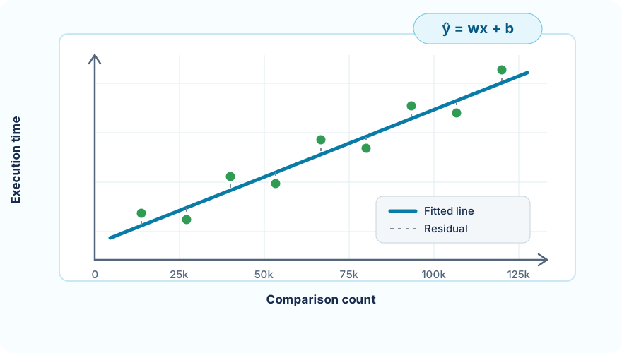
For one input feature, the model is:

• \(x\) is the input;
• \(w\) is the learned weight or slope;
• \(b\) is the learned bias or intercept;
• \(\hat{y}\) is the prediction.

The model learns the overall relationship instead of memorizing each row.

Why this is a neural network

A single Linear neuron calculates the same equation:

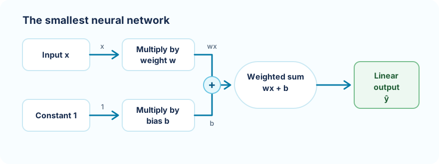
In Deep Netts this is a 1 -> 1 network: one input, no hidden layers, and one output with Linear activation. It is the smallest useful neural network.

Measure the error

For sample \(i\), the residual is:

Mean Squared Error averages squared residuals:

Squaring prevents positive and negative errors from cancelling and penalizes large misses more strongly.

Simple linear regression with Deep Netts

The runnable Sorting Execution Time walkthrough predicts execution_time_ms from comparison_count.

Load, shuffle, and split

TabularDataSet<MLDataItem> dataSet = DataSets.readCsv(
        DATASET_PATH, NUM_INPUTS, NUM_OUTPUTS, true, ",");

dataSet.shuffle(42);
TrainTestSplit split = dataSet.trainTestSplit(0.8);
DataSet<MLDataItem> trainingSet = split.getTrainingSet();
DataSet<MLDataItem> testSet = split.getTestSet();

The fixed seed makes the split reproducible. The test set remains unseen until evaluation.

Standardize the data

Standardizer standardizer = new Standardizer(trainingSet);
standardizer.apply(trainingSet);
standardizer.apply(testSet);

Fit preprocessing on training data only. Applying test statistics during training would leak information and make evaluation look more reliable than it is.

Build the model

FeedForwardNetwork neuralNet = FeedForwardNetwork.builder()
        .addInputLayer(NUM_INPUTS)
        .addOutputLayer(NUM_OUTPUTS, ActivationType.LINEAR)
        .lossFunction(LossType.MEAN_SQUARED_ERROR)
        .randomSeed(42)
        .build();

There is no hidden nonlinear transformation, so the network learns \(\hat{y}=wx+b\).

Train the model

neuralNet.getTrainer()
        .setStopEpochs(3000)
        .setLearningRate(0.001f)
        .setOptimizer(OptimizerType.SGD)
        .setShuffle(true);

neuralNet.train(trainingSet);

The learning rate controls update size. Too large can make loss unstable; too small can make learning unnecessarily slow.

Evaluate and predict

RegressionMetrics metrics = (RegressionMetrics) neuralNet.test(testSet);
System.out.println(metrics);

neuralNet.setNormalizer(standardizer);
float comparisonCount = 100_000;
float predictedExecutionTime = neuralNet.predict(comparisonCount)[0];

Attaching the fitted normalizer lets raw future inputs receive the same transformation used during training.

Training loss and held-out metrics answer different questions. Use the test metrics to judge generalization.

Multiple linear regression

With \(m\) features, the model becomes:

The Computer Hardware Performance walkthrough uses six inputs:

MYCT, MMIN, MMAX, CACH, CHMIN, CHMAX -> PRP

FeedForwardNetwork neuralNet = FeedForwardNetwork.builder()
        .addInputLayer(6)
        .addOutputLayer(1, ActivationType.LINEAR)
        .lossFunction(LossType.MEAN_SQUARED_ERROR)
        .randomSeed(42)
        .build();

The 6 -> 1 network still learns a linear relationship, now represented by a plane or hyperplane rather than a two-dimensional line.

Gradient descent

Training repeats:

1. create predictions with a forward pass;
2. calculate loss;
3. calculate each parameter's gradient;
4. update parameters in the direction that reduces loss.

For weight \(w\):

\(\eta\) is the learning rate. The gradient describes how the loss changes when the weight changes.

When a line is not enough

Linear regression cannot bend around a nonlinear relationship. Hidden layers with nonlinear activations change the model family:

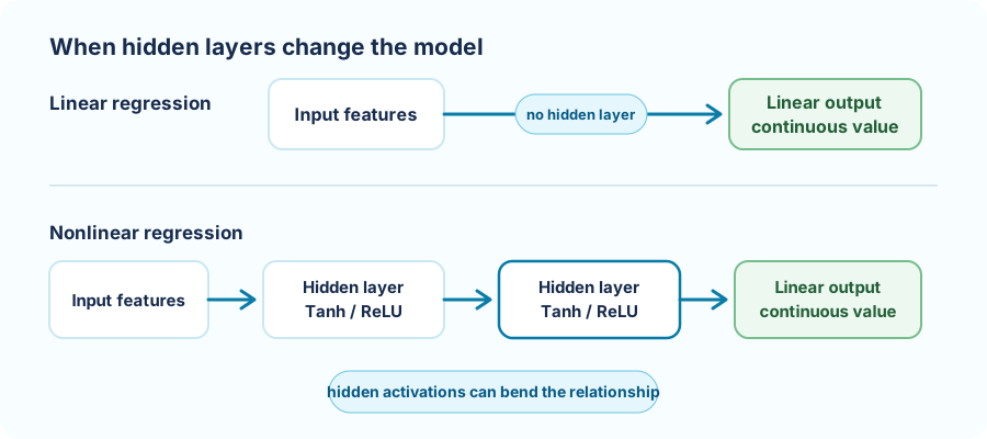
The House Price Prediction walkthrough demonstrates a 1 -> 16 -> 8 -> 1 nonlinear regression network.

Practical checklist

• Use regression for a continuous target.
• Keep feature order consistent.
• Split before fitting preprocessing.
• Use Linear activation at the regression output.
• Evaluate on held-out data using several metrics.
• Save preprocessing with the trained model.
• Add hidden layers only when a linear relationship is insufficient.

Looking for complete projects? Browse all Regression examples →

Continue learning

Turn a weighted linear score into a binary-class probability and decision boundary.

Next lessonLogistic Regression→