Logistic regression is a binary classifier: it predicts which of two classes a sample belongs to. It is the natural step between Linear Regression and multilayer Neural Networks because it keeps the same weighted linear calculation and changes how the result is interpreted.
Typical questions include:
Each problem has a target encoded with two possible values, commonly 0 and 1.
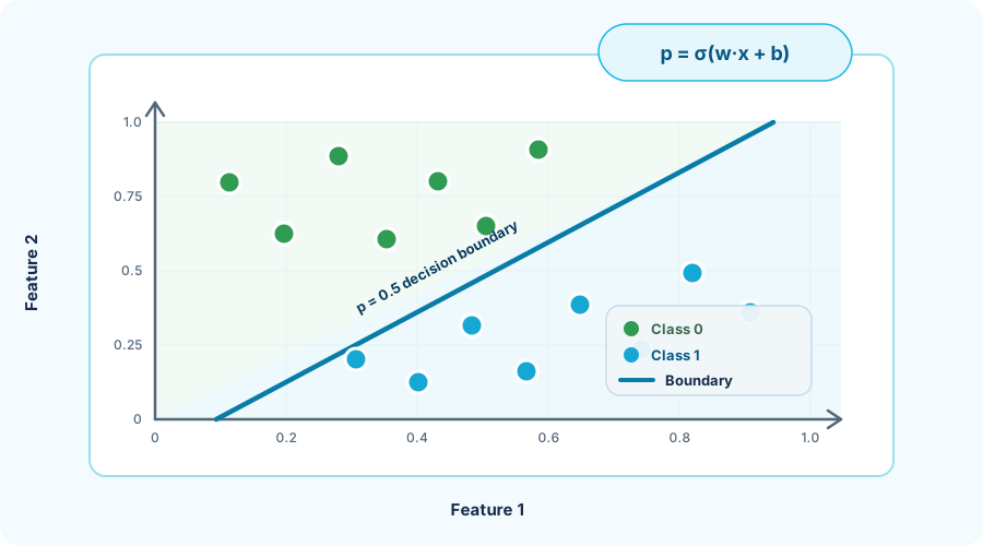
Linear regression predicts a continuous value. Binary classification instead needs a boundary that separates two classes.
For features \(x_1, x_2, \ldots, x_m\), the model first calculates the same weighted score used by linear regression:
The score \(z\) can be any real number. A Sigmoid activation converts it into a probability:
The result is always between 0 and 1:
1 indicates strong evidence for the positive class;0 indicates strong evidence for the negative class;0.5 represents the default decision boundary.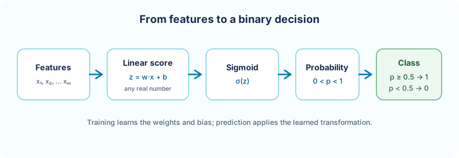
With a threshold of \(0.5\):
The probability is often more useful than the class alone because an application can choose a different threshold when false positives and false negatives have different costs.
Both models learn weights and a bias. Their output activations give the result a different meaning.
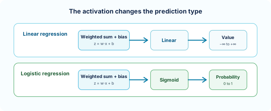
| Property | Linear Regression | Logistic Regression |
|---|---|---|
| Task | Predict a continuous value | Predict one of two classes |
| Output activation | Linear | Sigmoid |
| Output range | Any real number | Probability between 0 and 1 |
| Typical loss | Mean Squared Error | Cross-Entropy |
| Deep Netts output | One Linear value | One Sigmoid probability |
Logistic regression is also the smallest binary neural network. It has no hidden layer:
features -> weighted sum + bias -> Sigmoid -> probability
Without hidden layers, it can learn only a linear decision boundary. Hidden layers introduced in the next lesson allow a classifier to learn nonlinear boundaries.
The runnable Sonar Rock or Mine walkthrough applies logistic regression to 208 sonar observations. Each sample contains 60 numerical signal features and one binary target:
0 means ROCK;1 means MINE.Read the dataset with 60 inputs and one output:
TabularDataSet<MLDataItem> dataSet = DataSets.readCsv(
        DATASET_PATH, 60, 1, false, ",");
Shuffle deterministically and create separate training and test sets:
dataSet.shuffle(42);
TrainTestSplit split = dataSet.trainTestSplit(0.8);

DataSet<MLDataItem> trainingSet = split.getTrainingSet();
DataSet<MLDataItem> testSet = split.getTestSet();
Fit Min-Max scaling only on the training data, then apply the fitted scaler to the test set:
MinMaxScaler scaler = DataSets.scaleToMinMax(trainingSet);
scaler.apply(testSet);
This ordering prevents test information from leaking into preprocessing.
The model connects all 60 inputs directly to one Sigmoid output:
FeedForwardNetwork neuralNet = FeedForwardNetwork.builder()
        .addInputLayer(60)
        .addOutputLayer(1, ActivationType.SIGMOID)
        .lossFunction(LossType.CROSS_ENTROPY)
        .randomSeed(42)
        .build();
The absence of .addFullyConnectedLayer(...) is important: this is logistic regression, not a multilayer classifier.
Configure the trainer and learn the weights and bias:
neuralNet.getTrainer()
        .setStopEpochs(200)
        .setLearningRate(0.01f)
        .setOptimizer(OptimizerType.SGD)
        .setShuffle(true);

neuralNet.train(trainingSet);
Evaluate on samples that were not used to fit the model:
ClassificationMetrics metrics = (ClassificationMetrics) neuralNet.test(testSet);
System.out.println(metrics);
Classification metrics should be read together:
| Metric | Question it answers |
|---|---|
| Accuracy | How often is the classifier correct overall? |
| Precision | When it predicts the positive class, how often is it correct? |
| Recall | Of all actual positive samples, how many did it find? |
| F1 Score | How well are precision and recall balanced? |
| Specificity | How often does it correctly recognize the negative class? |
predict returns the positive-class probability. The application applies the threshold:
float mineProbability = neuralNet.predict(sonarSignal)[0];
String predictedClass = mineProbability >= 0.5f ? "MINE" : "ROCK";
The model returns evidence; the threshold turns that evidence into an application decision.
For one binary sample, Binary Cross-Entropy is:
\(y\) is the actual label and \(\hat{y}\) is the predicted probability. Across \(n\) samples, training minimizes the average:
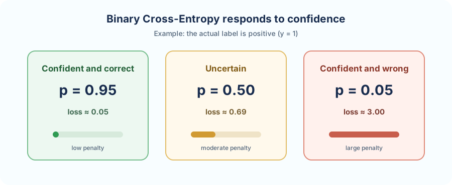
LossType.CROSS_ENTROPY.Sigmoid and Cross-Entropy form a useful pair. For logistic regression, their gradient simplifies to an error term multiplied by the feature value:
Gradient descent uses these derivatives to update every weight and the bias. The Backpropagation lesson develops this training process in detail.
The default threshold changes class when \(\sigma(z)=0.5\). Because \(\sigma(0)=0.5\), the boundary is:
With two features this equation describes a line. With three features it describes a plane, and with more features it describes a hyperplane.
This linear boundary is the model's main limitation. If the two classes require a curved or more complex separation, add hidden layers with nonlinear activation functions and use a neural-network classifier.
0 and 1.0.5 threshold, then tune it for application costs if necessary.Looking for complete projects? Browse all Classification examples →
Add hidden layers and learn nonlinear feature transformations.
To run the model from this lesson first, use the Sonar Rock or Mine walkthrough.
Was this helpful?
Thank you!