Convolutional Neural Networks

Convolutional Neural Networks (CNNs) are neural networks designed for data with spatial structure. In image classification, they learn local visual patterns and combine them into evidence for a class prediction.

A fully connected layer treats every input value as an independent position. A convolutional layer instead preserves image width, height, and channels while reusing the same small filter across many locations. This gives CNNs two useful properties:

local connectivity: a unit examines a small neighborhood rather than the entire image;
weight sharing: one learned filter detects the same pattern wherever it appears.

Images as tensors

An image enters a CNN as a three-dimensional tensor:

\[ H \times W \times C \]

\(H\) is height, \(W\) is width, and \(C\) is the number of channels. A grayscale image commonly has one channel; an RGB image has three. Resizing, channel order, and numerical scaling are part of the model input contract and must remain identical during training and prediction.

Convolution and feature maps

A convolutional filter is a small learned grid of weights. At each image location, it multiplies those weights by nearby input values, adds the results and a bias, then passes the value through an activation function.

For output channel \(k\) at location \((i,j)\):

\[ z_{i,j,k}=b_k+\sum_{u}\sum_{v}\sum_c w_{u,v,c,k}\,x_{i+u,j+v,c} \]

The activation map is then:

\[ a_{i,j,k}=f(z_{i,j,k}) \]

Each filter produces one feature map. During training, backpropagation changes the filter weights so useful patterns produce stronger responses.

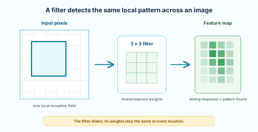
A three by three filter moving across local input pixels and producing a feature map — A filter reuses the same learned weights at every location, so one pattern detector can respond across the image.

Early filters often respond to simple local structures. Deeper layers combine earlier feature maps and can represent more complex shapes and object parts. The precise learned patterns come from the training objective rather than manual programming.

Filter size, stride, and padding

Three settings determine the spatial shape of a convolution:

filter size controls the local receptive field;
stride controls how far the filter moves between calculations;
padding adds values around the input boundary and can preserve more edge information.

For input size \(H\), filter size \(K\), padding \(P\), and stride \(S\), the output height is:

\[ H_{out}=\left\lfloor\frac{H+2P-K}{S}\right\rfloor+1 \]

The same calculation applies to width. Increasing stride or filter size generally reduces spatial resolution; padding can offset that reduction.

Activation and pooling

A nonlinear activation such as ReLU or Leaky ReLU follows convolution so stacked layers can learn nonlinear visual relationships.

Max pooling keeps the largest activation in each local window. It reduces width and height, lowers later computation, and retains a strong indication that a learned pattern was present. Pooling has no learned filter weights, but its window size and stride still affect information loss.

CNNs commonly repeat convolution and pooling before using fully connected layers for the final decision.

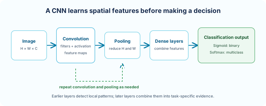
Image passing through convolution, activation, pooling, dense layers, and a classification output — Convolution extracts spatial features, pooling reduces their resolution, and dense layers combine them for a task-specific output.

Binary and multiclass outputs

The final layer follows the same rules introduced for other classifiers:

Image task	Output layer	Interpretation
Binary classification	One Sigmoid output	Probability of the positive class
Multiclass classification	One Softmax output per class	Probability distribution across classes

A Duke-logo detector can use one Sigmoid output. Handwritten-digit recognition requires ten Softmax outputs, one for each digit.

Build a CNN with Deep Netts

The Duke Logo example uses a compact binary architecture from the current Deep Netts API:

ConvolutionalNetwork network = ConvolutionalNetwork.builder()
        .addInputLayer(width, height, 3)
        .addConvolutionalLayer(6, Filters.ofSize(3))
        .addMaxPoolingLayer(2, 2)
        .addFullyConnectedLayer(16)
        .addOutputLayer(1, ActivationType.SIGMOID)
        .hiddenActivationFunction(ActivationType.LEAKY_RELU)
        .lossFunction(LossType.CROSS_ENTROPY)
        .randomSeed(42)
        .build();

The architecture reads as:

Builder call	Responsibility
`addInputLayer(width, height, 3)`	Declares RGB image dimensions
`addConvolutionalLayer(6, Filters.ofSize(3))`	Learns six local 3 × 3 filters
`addMaxPoolingLayer(2, 2)`	Reduces spatial dimensions
`addFullyConnectedLayer(16)`	Combines extracted features
`addOutputLayer(1, SIGMOID)`	Produces a binary probability

For a grayscale ten-class digit task, the input uses one channel and the output uses ten Softmax units. The runnable Handwritten Digit example also stacks two convolution-and-pooling stages.

Train and evaluate

CNN training still uses the backpropagation workflow from the previous lesson. The optimizer updates convolutional filters, dense weights, and biases from the same loss signal:

network.getTrainer()
        .setStopEpochs(epochs)
        .setLearningRate(0.001f)
        .setOptimizer(OptimizerType.ADAM)
        .setBatchMode(true)
        .setBatchSize(8)
        .setShuffle(true);

network.train(trainingSet);
System.out.println(network.test(testSet));

Evaluate on images excluded from training. Accuracy alone may hide class imbalance, so inspect precision, recall, F1, specificity, and the confusion matrix when the cost of errors differs between classes.

Design and debugging checklist

Preserve image size, channel count, channel order, and scaling.
Shuffle and split before training; do not evaluate on training images.
Match Sigmoid or Softmax to the target representation.
Begin with a compact architecture and add capacity only when evidence supports it.
Watch training and test behavior for overfitting.
Use augmentation only on training images and keep transformations realistic.
Save the image preprocessing contract with the trained network.
Release the network thread pool when the application finishes.

Runnable image examples

Browse the complete Image Classification examples gallery →

Duke Logo Recognition demonstrates a compact binary CNN.
Handwritten Digit Recognition demonstrates a deeper multiclass CNN.
Hot Dog or Not Hot Dog connects a binary image dataset to a complete training workflow.
TensorFlow VGGNet16 Import shows a much deeper pretrained architecture without presenting it as a beginner training task.

Continue learning

Connect datasets, model builders, trainers, metrics, saving, and prediction across tabular and image models.

Next lessonDeep Netts API

Was this helpful?

Table Of Contents