Backpropagation

When neuralNet.train(trainingSet) runs, Deep Netts performs a forward pass, calculates loss, propagates gradients backward, and updates every trainable weight and bias. Backpropagation is the algorithm that calculates those gradients.

The learning loop

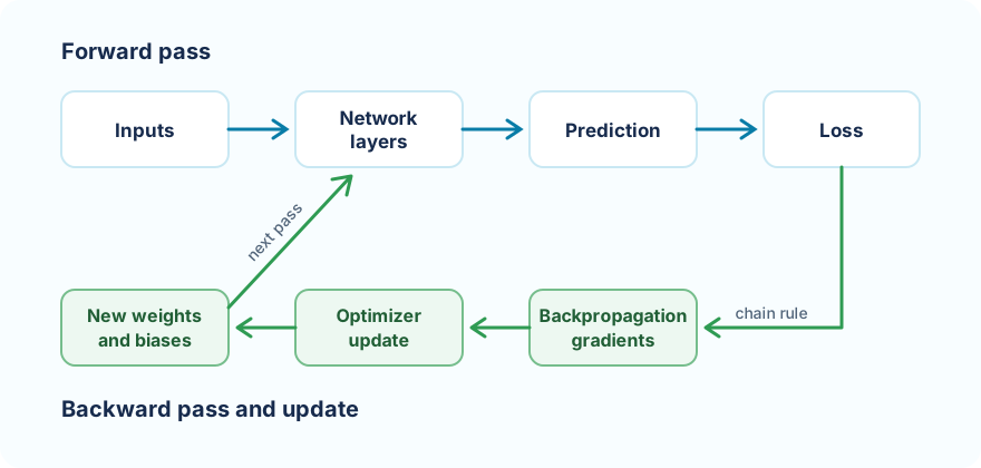
The network is not told the correct weights. It learns through many small parameter changes that reduce prediction error.

Forward pass

A neuron calculates a weighted sum and activation:

Each layer's activations become the next layer's inputs. The output layer produces a numerical value or class probabilities.

Loss functions

Loss converts prediction quality into one value the trainer can minimize.

Mean Squared Error

Regression commonly uses:

.lossFunction(LossType.MEAN_SQUARED_ERROR)

Cross-entropy

Classification commonly uses:

.lossFunction(LossType.CROSS_ENTROPY)

Cross-entropy works naturally with Sigmoid or Softmax probability outputs.

Backward pass

Backpropagation moves from the loss toward earlier layers. A gradient answers: if this parameter changed slightly, how would the loss change?

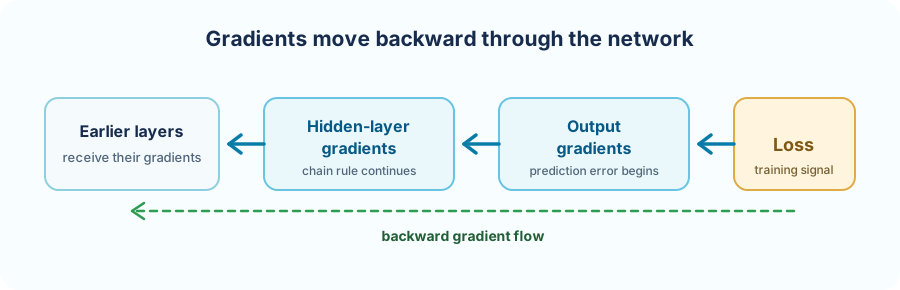
Backpropagation supplies gradients. The optimizer uses them to change parameters.

Chain rule

Neural networks are nested functions. For \(L(f(g(x)))\):

For one output neuron:

the weight gradient is:

The same pattern repeats through all layers. Forward-pass values are reused during the backward pass.

Optimizer and learning rate

Basic gradient descent updates parameter \(\theta\) with:

\(\eta\) is the learning rate.

neuralNet.getTrainer()
        .setStopEpochs(1000)
        .setLearningRate(0.001f)
        .setOptimizer(OptimizerType.SGD)
        .setShuffle(true);

The current API configures training through neuralNet.getTrainer(). Older snippets using BackpropagationTrainer, setMaxEpochs, setInput, or getOutput should not be copied into Deep Netts 4 projects.

Epochs and batches

An epoch is one pass through the training dataset. Depending on configuration, updates can happen for individual samples or batches.

epoch 1: visit rows -> gradients -> updates
epoch 2: reshuffle  -> gradients -> updates
...

setStopEpochs is an upper limit. Training can finish earlier when another stopping condition is satisfied. Shuffling reduces the influence of row order.

Current Deep Netts classification flow

The following structure matches the runnable Iris Flower walkthrough.

Load and split

TabularDataSet<MLDataItem> dataSet = DataSets.readCsv(
        DATASET_PATH, NUM_INPUTS, NUM_OUTPUTS, true, ",");

dataSet.shuffle(42);
TrainTestSplit split = dataSet.trainTestSplit(0.8);
DataSet<MLDataItem> trainingSet = split.getTrainingSet();
DataSet<MLDataItem> testSet = split.getTestSet();

Fit preprocessing without leakage

MinMaxScaler scaler = DataSets.scaleToMinMax(trainingSet);
scaler.apply(testSet);

Build the network

FeedForwardNetwork neuralNet = FeedForwardNetwork.builder()
        .addInputLayer(4)
        .addFullyConnectedLayer(16, ActivationType.TANH)
        .addOutputLayer(3, ActivationType.SOFTMAX)
        .lossFunction(LossType.CROSS_ENTROPY)
        .randomSeed(42)
        .build();

Train and evaluate

neuralNet.getTrainer()
        .setStopError(0.03f)
        .setStopEpochs(350)
        .setLearningRate(0.001f)
        .setOptimizer(OptimizerType.ADAM);

neuralNet.train(trainingSet);
ClassificationMetrics metrics =
        (ClassificationMetrics) neuralNet.test(testSet);

Training output measures optimization on the training subset. ClassificationMetrics evaluates unseen examples.

Learning-rate experiments

Change one variable at a time and create a fresh network for every experiment:

float[] learningRates = {0.0001f, 0.001f, 0.01f};

for (float learningRate : learningRates) {
    FeedForwardNetwork neuralNet = buildNetwork();
    neuralNet.getTrainer()
            .setStopEpochs(1000)
            .setLearningRate(learningRate)
            .setOptimizer(OptimizerType.SGD)
            .setShuffle(true);
    neuralNet.train(trainingSet);
}

Reusing an already trained network would invalidate the comparison.

Architecture experiments

Backpropagation works for linear and multilayer models:

linear:     4 -> 3
one hidden: 4 -> 16 -> 3
two hidden: 4 -> 16 -> 8 -> 3

For a fair comparison, keep the split, preprocessing, random seed, optimizer, learning rate, and stopping rules equal. Compare held-out metrics rather than training loss alone. More layers add capacity but can overfit small datasets.

Activation derivatives

For Sigmoid:

For Tanh:

For ReLU away from zero:

These derivatives become factors in the chain rule.

Vanishing and exploding gradients

Multiplying many derivatives smaller than one can leave early layers with an almost-zero gradient. This is the vanishing-gradient problem. Repeatedly large factors can produce exploding gradients.

Practical responses include:

• scale numerical inputs;
• use suitable activations such as ReLU in deeper hidden layers;
• choose a conservative learning rate;
• avoid unnecessary depth;
• monitor loss for instability and non-finite values.

Diagnose training

• Falling error shows progress on training data.
• Flat error can mean convergence, weak gradients, or unsuitable settings.
• Oscillation often indicates an excessive learning rate.
• Strong training results with weak test metrics suggest overfitting.
• Regression “accuracy” can be negative early in training; interpret it with regression loss and held-out metrics.

Practical checklist

• Match output activation and loss to the task.
• Split before fitting preprocessing.
• Use reproducible seeds for comparisons.
• Change one experimental variable at a time.
• Treat epoch count as an upper limit when other stopping rules exist.
• Evaluate on held-out data.
• Save preprocessing with the trained model.

Continue learning

See how the same training process learns reusable spatial filters for images.

Next lessonConvolutional Neural Networks→