Neural Networks

A neural network is a model that transforms input features into a prediction. Before looking at individual neurons and equations, it is more useful to understand the network as a complete system.

For a Java developer, the high-level idea resembles a processing pipeline:

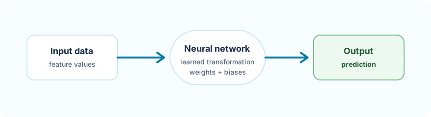
Input feature data passing through a neural network model to produce an output prediction — A neural network receives a defined set of feature values, applies its learned transformations, and returns a prediction.

The model has an expected input structure, performs a sequence of transformations, and returns a result. Training determines the internal parameters used by those transformations.

Complete prediction flow

Consider the email spam example. One email is represented by five numerical features:

num_links
num_words
has_offer
sender_score
all_caps

The complete prediction flow is:

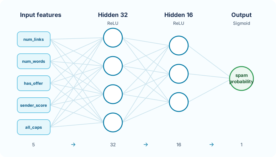
Five email features passing through two hidden layers to a spam-probability output — The architecture describes both the input contract and the transformations that lead to one Sigmoid probability.

At this level, the network can be treated as a function:

five input values -> one output value

The output is a number between 0 and 1. A threshold such as 0.5 converts it into a class.

This input-to-output contract is the first thing to understand. The internal structure explains how the model performs the transformation.

Read the architecture

The spam network has this architecture:

5 -> 32 -> 16 -> 1

Each number describes the size of one layer:

5 input values,
32 neurons in the first hidden layer,
16 neurons in the second hidden layer,
1 output value.

Data flows forward through the complete network shown above: from five input features, through 32 and 16 ReLU hidden neurons, to one Sigmoid probability.

The notation provides a compact system-level view before we inspect what happens inside each layer.

Layer responsibilities

A feed-forward network organizes its transformations into layers.

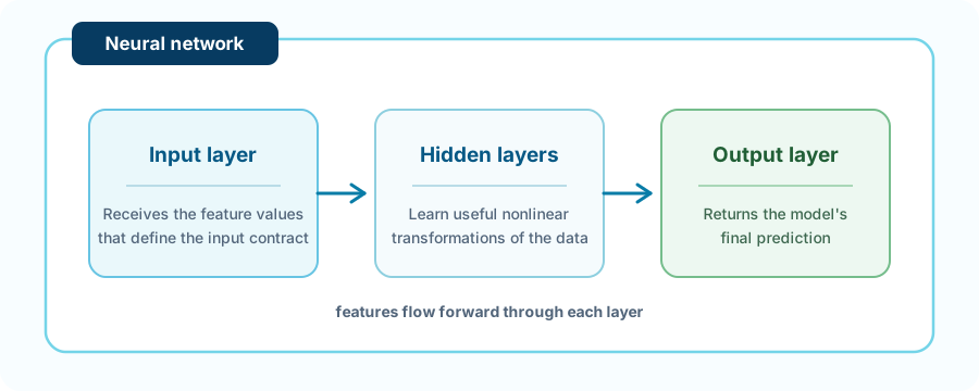
The input layer defines what enters the model, hidden layers learn useful transformations, and the output layer returns the prediction.

Input layer: define the model contract

The input layer receives feature values. Its size must match the number of features supplied for each sample.

In the spam example, five dataset columns become five network inputs. The feature order is part of the contract: changing the order changes the meaning of the data.

Hidden layers: transform representations

Hidden layers sit between the input and output. Each hidden layer receives values from the preceding layer and produces a new representation for the following layer.

The spam network uses layers of 32 and 16 neurons. These layers allow the model to learn non-linear combinations of email characteristics. A pattern may depend on several features together rather than on one feature alone.

A network can have no hidden layers, one hidden layer, or several hidden layers. More layers and neurons create more trainable parameters and greater capacity, but they may also require more data and careful training.

The Logistic Regression lesson demonstrates the zero-hidden-layer case with the runnable Sonar walkthrough. Its 60 -> 1 architecture learns a linear decision boundary, while the Spam network uses hidden layers to learn non-linear feature combinations.

Output layer: match the prediction task

The output layer returns the final prediction. Its structure depends on the problem:

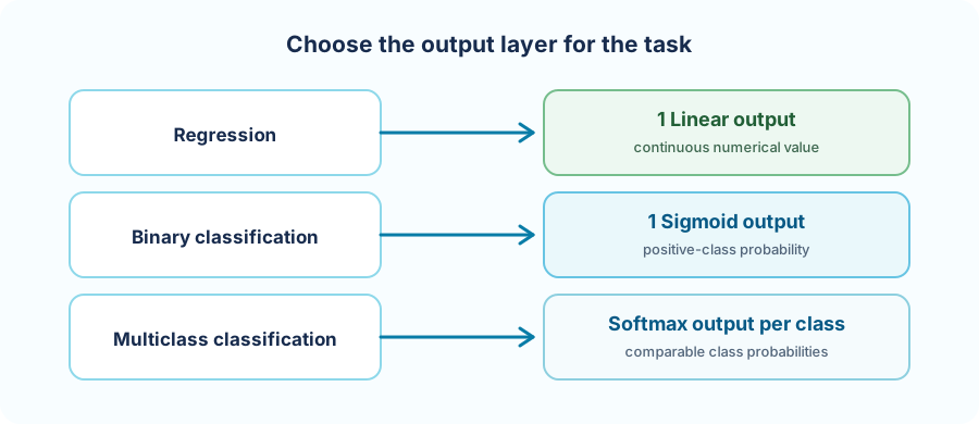
Regression mapped to one Linear output, binary classification to one Sigmoid output, and multiclass classification to one Softmax output per class — The prediction task determines the output size and activation function.

The spam classifier uses one Sigmoid output because it predicts the probability of one positive class: spam.

The Iris classifier uses three Softmax outputs. Together they represent the probabilities of SETOSA, VERSICOLOR, and VIRGINICA.

Compare network designs

These four examples demonstrate how architecture follows the prediction problem.

Problem	Example	Features	Architecture	Output	Walkthrough
Binary classification	Spam classifier	5 email features	`5 → 32 → 16 → 1`	1 Sigmoid probability	View example →
Multiclass classification	Iris classifier	4 flower measurements	`4 → 16 → 3`	3 Softmax probabilities	View example →
Image classification	Hot Dog classifier	RGB image pixels	`convolution → pooling → fully connected`	1 Sigmoid probability	View example →
Multiple linear regression	Computer Hardware predictor	6 hardware features	`6 → 1`	1 Linear value	View example →

At the system level, all of these models have the same responsibility:

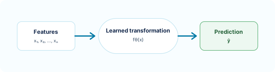
Input features passing through a learned model transformation to produce a prediction — Different architectures learn different transformations, but every predictive model maps an agreed input contract to an output.

Their internal structures differ because they solve different kinds of prediction problems.

Inside one neuron

After understanding the network and its layers, we can inspect the smallest computational unit.

A neuron receives values from the preceding layer. Each value is multiplied by a weight, the weighted values are added, and a bias is included:

weighted sum = x1*w1 + x2*w2 + ... + xn*wn + bias

Where:

x1 ... xn are values entering the neuron,
w1 ... wn are trainable weights,
bias is an additional trainable value.

The weights control how strongly each incoming value affects the result. The bias allows the neuron to shift its result independently of those inputs.

One neuron performs a small calculation. A layer performs many such calculations, and the network composes the transformations of all its layers.

Activation functions

After calculating its weighted sum, a neuron usually applies an activation function:

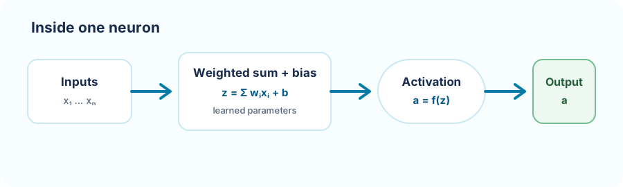
Neuron inputs entering a weighted sum with bias, followed by an activation function and output — A neuron first combines its inputs with learned weights and a bias, then applies an activation function to the result.

Common activation functions have different responsibilities:

Activation	Typical role
Linear	Predicting an unrestricted numerical value
ReLU	Learning non-linear patterns in hidden layers
Sigmoid	Producing a value between `0` and `1`

Plots comparing Linear, ReLU, and Sigmoid activation functions — Linear preserves the full numerical range, ReLU introduces a simple non-linearity, and Sigmoid compresses its output into a probability-like value between 0 and 1.

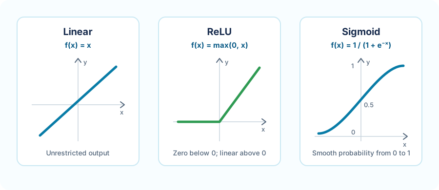
The spam network uses ReLU in its hidden layers and Sigmoid in its output layer. The regression network uses a Linear output.

Without non-linear activation functions in hidden layers, stacking several layers would still behave like a single linear transformation. Non-linearity allows hidden layers to represent more complex relationships.

How training works

Defining the architecture creates an untrained network. Its initial weights and biases do not yet represent useful patterns in the dataset.

Training repeatedly performs this high-level loop:

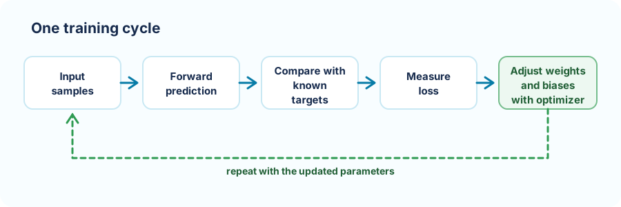
Training cycle from input samples and forward prediction to loss measurement and parameter adjustment — Each cycle uses the current parameters to make predictions, measures their error, and produces updated weights and biases for the next pass.

In more specific terms, training:

sends samples forward through the complete network,
compares predictions with known targets,
measures the error using a loss function,
uses backpropagation and an optimizer to adjust parameters.

The network architecture remains the same during this process. What changes are the learned weights and biases inside its neurons.

From loss to a parameter update

One training update connects four operations:

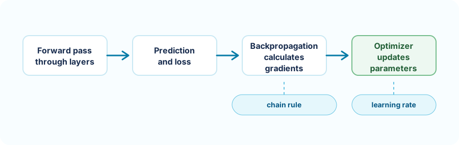
Forward pass, prediction and loss, backpropagation gradients, and optimizer parameter update — Backpropagation calculates gradients with the chain rule; the optimizer combines those gradients with the learning rate to update the parameters.

A gradient describes how the loss would change if one parameter changed slightly. Backpropagation moves from the output toward earlier layers and applies the chain rule to calculate a gradient for every trainable weight and bias.

The optimizer then uses those gradients. The simplest update is gradient descent:

new weight = old weight - learning rate * gradient

The learning rate controls the size of each step. If it is too large, loss may oscillate or diverge. If it is too small, training may improve so slowly that it does not converge within the chosen epoch limit.

Epochs, batches, and updates

An epoch is one complete pass through the training set. A batch is the group of samples used to calculate one parameter update.

For 1,000 samples and a batch size of 100:

1 epoch = 10 batches = 10 parameter updates

Smaller batches update the model more frequently and introduce useful variation, while larger batches produce smoother estimates but require more memory. Epoch count and batch size are hyperparameters: neither is learned by the network.

Why ReLU helps deeper networks

Backpropagation multiplies derivatives while moving through layers. With many Sigmoid or Tanh layers, these values can repeatedly shrink until early layers receive an almost-zero gradient. This is the vanishing gradient problem.

ReLU is commonly used in hidden layers because its positive-side derivative does not shrink the gradient in the same way. It does not eliminate every training difficulty, but it is one reason ReLU is a practical default for deeper feed-forward and convolutional networks.

Count model parameters

For two consecutive fully connected layers, the parameter count is:

parameters = inputs * outputs + output biases

For the Iris architecture 4 -> 16 -> 3:

input to hidden: 4 * 16 + 16 = 80
hidden to output: 16 * 3 + 3 = 51
total: 131 trainable parameters

More parameters increase model capacity, but they also increase memory use and the risk of overfitting. Parameter count therefore helps compare architectures more meaningfully than layer count alone.

Architecture decisions

Choosing an architecture involves deciding:

how many input features the model receives,
whether the problem needs hidden layers,
how many neurons each hidden layer contains,
which activation functions match each layer's role,
how many outputs the prediction requires.

There is no single best architecture for every dataset. Begin with the smallest model that matches the problem, evaluate it, and increase complexity only when the evidence supports doing so.

The important top-down questions are:

What enters the model?
What should it predict?
Which layers transform the data?
What does each neuron do inside those layers?
How does training improve the complete system?

Continue learning

See how loss gradients flow backward through these layers and update every trainable parameter.

Next lessonBackpropagation

Frequently Asked Questions

What does a neuron compute?

A neuron combines weighted inputs with a bias and passes the result through an activation function.

Why are hidden layers useful?

Hidden layers build intermediate representations that let a network learn nonlinear relationships and increasingly complex patterns.

Was this helpful?

Table Of Contents