Natural Language Processing

Natural Language Processing (NLP) applies Machine Learning to text and language. It turns documents, sentences, or token sequences into numerical representations that a model can use for classification, scoring, extraction, similarity, or generation.

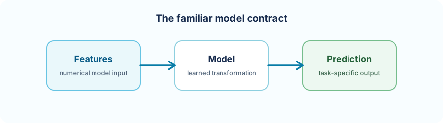
NLP is not a separate replacement for the workflow developed earlier in the course. It adds a language-specific preparation stage before the familiar sequence:

From language to model input

A model cannot consume the meaning of raw text directly. The application first decides which parts of the text matter and how to represent them numerically.

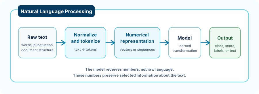
Every stage defines part of the model contract:

• Raw text — The original language input includes words, case, punctuation, accents, formatting, and document structure that may carry useful information.
• Normalize and tokenize — Normalization decides which details are preserved or transformed, while tokenization defines the basic units, such as words, subwords, characters, punctuation, or special markers.
• Numerical representation — A vocabulary maps known tokens to stable identifiers or feature positions, and the selected representation converts them into vectors or numerical sequences.
• Model — The model learns transformations from the prepared numerical input rather than operating on raw language directly.
• Output — The final representation is converted into the result required by the task, such as a class, score, token label, ranked match, or generated text.

Changing any of these decisions after training changes what the model receives.

Tokens and vocabulary

A token is one unit processed by the language pipeline. Depending on the tokenizer, a token may be a word, part of a word, punctuation mark, character, or special marker.

For a small educational word tokenizer, plain Java might normalize and split text like this:

String normalized = text
        .toLowerCase(Locale.ROOT)
        .replaceAll("[^\\p{L}\\p{N}']+", " ")
        .trim();

List<String> tokens = normalized.isEmpty()
        ? List.of()
        : List.of(normalized.split("\\s+"));

This snippet is intentionally simple. Production tokenization must define behavior for languages, Unicode, contractions, URLs, numbers, emoji, markup, and unknown tokens.

A vocabulary gives each known token a stable index:

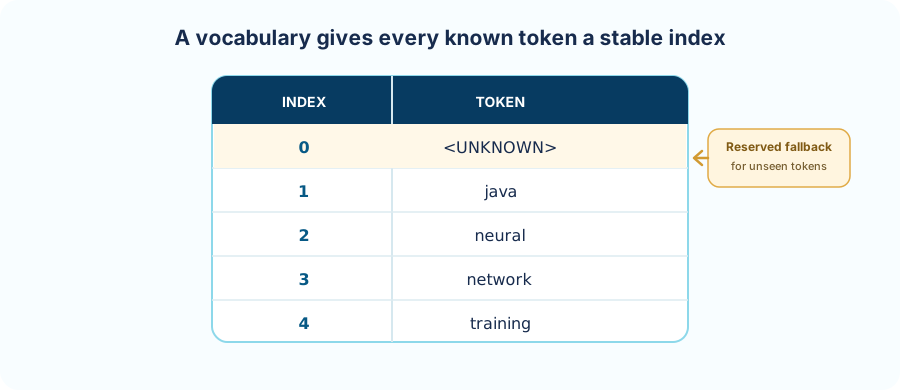
Unknown or rare tokens are commonly mapped to a reserved value instead of silently changing the input shape.

Numerical text representations

The representation determines what the model can learn from the text.

Bag of Words

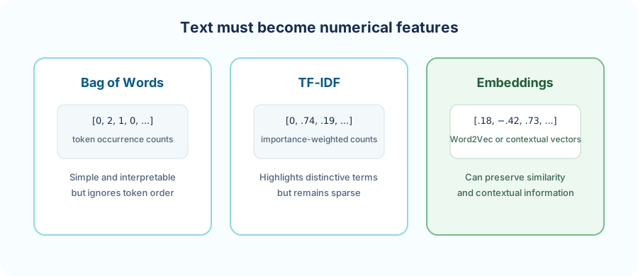
Bag of Words creates one feature per vocabulary term and stores a count or presence value. It is simple and interpretable, but it discards token order.

For vocabulary \(V\) and document \(d\), feature \(j\) is the number of times vocabulary term \(V_j\) occurs in that document:

Consider this training corpus:

• \(D_1\): java neural network
• \(D_2\): java network training
• \(D_3\): java virtual machine

The vocabulary fixes the column order: java, neural, network, training, virtual, machine. Each document then becomes a vector of counts.

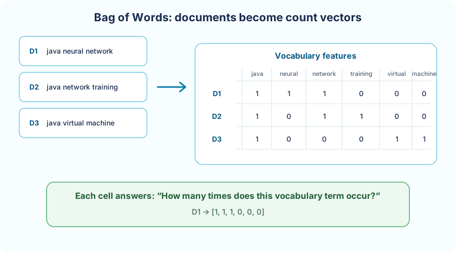
The vocabulary must be fitted on the training set and reused unchanged for test and future documents. A term outside that vocabulary needs an explicit policy, such as an unknown-token feature or omission.

TF-IDF

Raw counts can overemphasize words that occur throughout the corpus. Term Frequency–Inverse Document Frequency separates the calculation into three parts.

1. Term frequency (TF) measures how prominent term \(t\) is inside document \(d\):

\(|d|\) is the number of tokens in the document. Dividing by document length makes counts from documents of different sizes easier to compare.

2. Inverse document frequency (IDF) measures how distinctive the term is across the training corpus:

\(N\) is the number of training documents, while \(\operatorname{df}(t)\) is the number of those documents containing \(t\). A term found in fewer documents receives a larger IDF value.

3. TF-IDF combines local prominence and corpus-wide distinctiveness:

For neural in \(D_1\), \(\operatorname{tf}=1/3\), \(\operatorname{idf}=\ln(3/1)\), and the resulting TF-IDF weight is approximately \(0.366\). By contrast, java occurs in every document, so this unsmoothed formula gives it an IDF of zero.

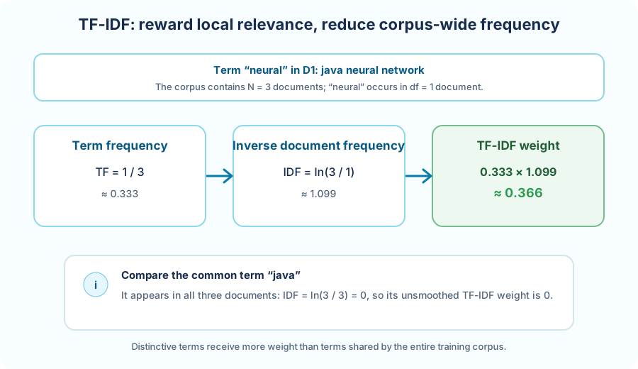
This is the clearest educational form of TF-IDF. Production libraries may add smoothing, use another logarithm base, apply sublinear TF, and normalize the final vector. Whichever variant is selected becomes part of the model contract and must remain identical during training and prediction.

Embeddings

An embedding maps a token, sentence, or document to a dense numerical vector. Similar language units can occupy nearby regions of the learned vector space.

Word2Vec

Word2Vec is a family of shallow neural models that learns one dense vector for every word in a vocabulary. Instead of using a manually assigned meaning, it learns from context: words that occur in similar surroundings tend to receive nearby vectors.

Training examples are created by sliding a fixed-size context window through a text corpus. Word2Vec can then use either of two learning objectives:

• Continuous Bag of Words (CBOW) receives the surrounding context words and predicts the word in the center;
• Skip-gram receives the center word and predicts its surrounding context words.

For the fragment java neural network training, a CBOW example could use java and network to predict neural. A Skip-gram example reverses that relationship and uses neural to predict nearby words such as java and network.

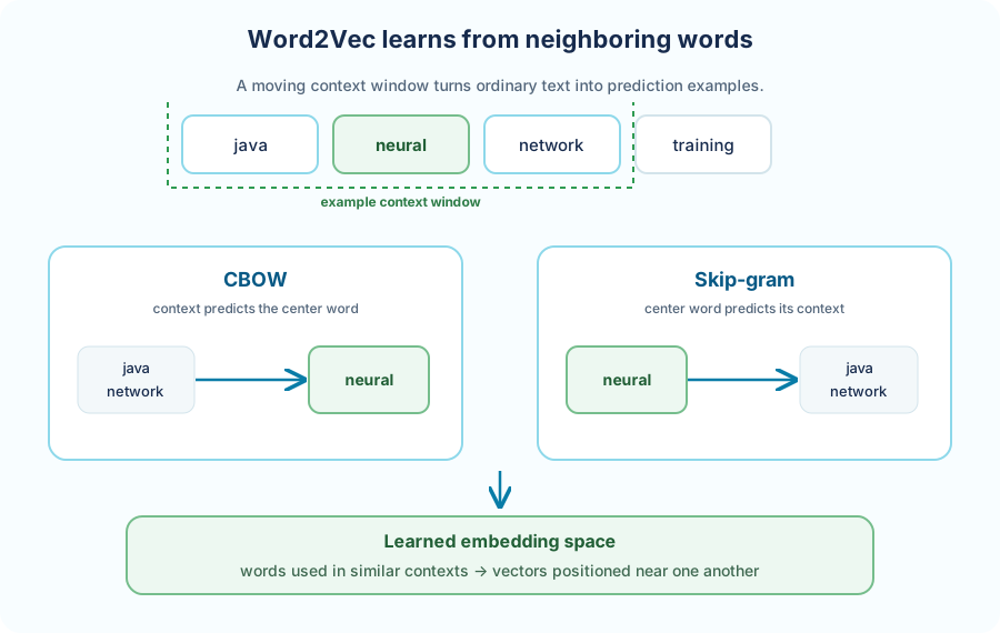
The trained hidden-layer weights become the word vectors. Their useful dimensions are learned rather than named manually, and vector similarity—often cosine similarity—can be used to find words that occur in related contexts.

Word2Vec produces static embeddings: java receives the same vector in every sentence. Contextual models can instead produce a different representation according to the surrounding text.

What can an embedding represent?

The same general idea—representing an item with a dense vector—extends beyond individual words:

High-dimensional embeddings can be projected into two dimensions with methods such as t-SNE for exploratory visualization. A visible cluster can suggest similar representations, but the projection distorts some distances and is not a substitute for task-specific evaluation.

Embeddings used by an NLP application may be:

• learned together with a task-specific model;
• produced by a separately trained model;
• supplied by an external embedding service.

An external embedding model or service is not an integrated Deep Netts feature unless the application connects and validates it explicitly.

Common NLP tasks

The first four tasks analyze existing text. Language modeling and generation predict or create new sequences and lead directly into Generative AI.

Text classification with Deep Netts

Once text has become a fixed numerical feature vector, a Deep Netts classifier can use the same API pattern as other tabular examples.

For a binary document classifier with NUM_TEXT_FEATURES prepared inputs:

FeedForwardNetwork classifier = FeedForwardNetwork.builder()
        .addInputLayer(NUM_TEXT_FEATURES)
        .addFullyConnectedLayer(32, ActivationType.RELU)
        .addOutputLayer(1, ActivationType.SIGMOID)
        .lossFunction(LossType.CROSS_ENTROPY)
        .randomSeed(42)
        .build();

The model sees only numbers. The application must preserve:

• the exact vocabulary and token-to-index mapping;
• the same normalization and tokenizer rules;
• the same vectorization and scaling behavior;
• the feature order used during training;
• the class mapping and decision threshold.

The runnable Email Spam Detection walkthrough demonstrates the classification, training, metrics, saving, and prediction stages. Its five inputs are prepared email and sender characteristics, so it is a useful classifier reference but not a raw-text NLP pipeline.

Sequence order and context

Bag-of-Words and TF-IDF summarize a document into one fixed vector. Some tasks instead require token order and long-range context.

Fixed-vector models

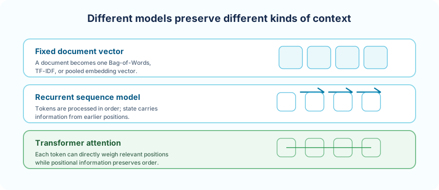
A feed-forward classifier can work well when a fixed representation already captures enough evidence. It is often a strong baseline for topic, spam, intent, or sentiment classification.

Recurrent models

Recurrent Neural Networks process a sequence step by step and carry a hidden state forward. LSTM and GRU variants add gates that help retain useful information across longer ranges.

Transformers

Transformers use self-attention so each token representation can combine information from relevant positions. Positional information preserves order, while multi-head attention learns several relationships in parallel.

These sequence-aware architectures are explained conceptually here. The current cookbook does not present them as runnable built-in Deep Netts examples.

Developing a trustworthy NLP model

Text pipelines introduce additional leakage and evaluation risks.

Split documents before fitting

Create training, validation, and test document groups before:

• selecting vocabulary terms;
• calculating document frequencies for TF-IDF;
• learning task-specific embeddings;
• selecting thresholds or hyperparameters.

Near-duplicate documents, quoted text, message threads, or documents from the same author can leak information across random splits. Group-based or time-based splits may better represent production behavior.

Evaluate the task, not only the loss

For classification, inspect accuracy, precision, recall, F1, specificity, and the confusion matrix. For retrieval, use ranking metrics. For generated text, automated metrics alone are rarely sufficient; quality, grounding, safety, and human review may also matter.

Preserve the complete text contract

Saving only the neural network is insufficient. A deployable NLP system must also preserve tokenizer configuration, vocabulary, representation settings, class names, thresholds, and any external model or service version.

Practical checklist

• Define the language task and target before selecting an architecture.
• Decide what one sample represents: message, sentence, document, or token sequence.
• Split documents before fitting vocabulary or corpus statistics.
• Normalize and tokenize training and future text identically.
• Start with an interpretable fixed-vector baseline when appropriate.
• Use a sequence-aware model only when order and context materially matter.
• Evaluate class-specific errors and dataset leakage.
• Version every preprocessing and external-model dependency with the trained model.
• Do not represent an external embedding or LLM service as built-in Deep Netts functionality.

Continue learning

See how next-token prediction, Transformer attention, sampling, and external LLM integration extend these NLP foundations into text generation.

Next lessonGenerative AI Optional→